
 E-mail Alert
 RSS
RSS
| Citation: |

|
Blind restoration of atmospheric turbulence degraded images by sparse prior model
-
Abstract
Blind image deconvolution is one method of restoring both kernel and real sharp image only from degraded images, due to its illness, image priors are necessarily applied to constrain the solution. Given the fact that traditional image gradient l2 and l1 norm priors cannot describe the gradient distribution of natural images, in this paper, the image sparse prior is applied to the restoration of single-frame atmospheric turbulence degraded images. Kernel estimation is performed first, followed by non-blind restoration and the split Bregman algorithm is used to solve the non-convex cost function. Simulation results show that compared with total variation priori, sparse priori is better at kernel estimation, producing sharp edges and removal of ringing, etc., which reducing the kernel estimation error and improving restoration quality. Finally, the real turbulence-degraded images are restored.-
Keywords:
- adaptive optics /
- sparse prior /
- blind deconvolution /
- split Bregman
-

-
References
[1] 姜文汉.自适应光学技术[J].自然杂志, 2006, 28(1): 7-13. doi: 10.3969/j.issn.0253-9608.2006.01.002 Jiang W H. Adaptive optical technology[J]. Chinese Journal of Nature, 2006, 28(1): 7-13. doi: 10.3969/j.issn.0253-9608.2006.01.002 [2] 鲍华, 饶长辉, 田雨, 等.自适应光学图像事后重建技术研究进展[J].光电工程, 2018, 45(3): 58-67. doi: 10.12086/oee.2018.170730 Bao H, Rao C H, Tian Y, et al. Research progress on adaptive optical image post reconstruction[J]. Opto-Electronic Engineering, 2018, 45(3): 58-67. doi: 10.12086/oee.2018.170730 [3] Levin A, Weiss Y, Durand F, et al. Understanding and evaluating blind deconvolution algorithms[C]//Proceedings of 2009 IEEE conference on Computer Vision and Pattern Recognition, Miami, 2009: 1964-1971. [4] Perrone D, Favaro P. Total variation blind deconvolution: the devil is in the details[C]//Proceedings of 2014 IEEE Conference on Computer Vision and Pattern Recognition, Columbus, 2014: 2909-2916. [5] Ayers G R, Dainty J C. Iterative blind deconvolution method and its applications[J]. Optics Letters, 1988, 13(7): 547-549. doi: 10.1364/OL.13.000547 [6] Lane R G. Blind deconvolution of speckle images[J]. Journal of the Optical Society of America A, 1992, 9(9): 1508-1514. doi: 10.1364/JOSAA.9.001508 [7] Jefferies S M, Christou J C. Restoration of astronomical images by iterative blind deconvolution[J]. Astrophysical Journal, 1993, 415(2): 862-874. [8] You Y L, Kaveh M. A regularization approach to joint blur identification and image restoration[J]. IEEE Transactions on Image Processing, 1996, 5(3): 416-428. [9] Chan T F, Wong C K. Total variation blind deconvolution[J]. IEEE Transactions on Image Processing, 1998, 7(3): 370-375. [10] Fergus R, Singh B, Hertzmann A, et al. Removing camera shake from a single photograph[J]. ACM Transactions on Graphics, 2006, 25(3): 787-794. doi: 10.1145/1141911.1141956 [11] Krishnan D, Tay T, Fergus R. Blind deconvolution using a normalized sparsity measure[C]//Proceedings of the 24th IEEE Conference on Computer Vision and Pattern Recognition, Providence, 2011: 233-240. [12] Kotera J, Šroubek F, Milanfar P. Blind deconvolution using alternating maximum a posteriori estimation with heavy-tailed priors[C]//Proceedings of the 15th International Conference on Computer Analysis of Images and Patterns, York, 2013: 59-66. [13] Goldstein T, Osher S. The split bregman method for L1-regularized problems[J]. SIAM Journal on Imaging Sciences, 2009, 2(2): 323-343. doi: 10.1137/080725891 [14] Krishnan D, Fergus R. Fast image deconvolution using hyper-Laplacian priors[C]//Proceedings of the 22nd International Conference on Neural Information Processing Systems, Vancouver, 2009: 1033-1041. [15] Chan T F, Wong C K. Convergence of the alternating minimization algorithm for blind deconvolution[J]. Linear Algebra and its Applications, 2000, 316(1-3): 259-285. doi: 10.1016/S0024-3795(00)00141-5 [16] Levin A, Fergus R, Durand F, et al. Image and depth from a conventional camera with a coded aperture[J]. ACM Transactions on Graphics, 2007, 26(3): 70. doi: 10.1145/1276377.1276464 [17] 王齐涛, 佟首峰, 徐友会.采用Zernike多项式对大气湍流相位屏的仿真和验证[J].红外与激光工程, 2013, 42(7): 1907-1911. doi: 10.3969/j.issn.1007-2276.2013.07.046 Wang Q T, Tong S F, Xu Y H. On simulation and verification of the atmospheric turbulent phase screen with Zernike polynomials[J]. Infrared and Laser Engineering, 2013, 42(7): 1907-1911. doi: 10.3969/j.issn.1007-2276.2013.07.046 -
Overview

Overview: Atmospheric turbulence is a major factor limiting the imaging resolution of ground-based telescopes. Adaptive optics (AO) is commonly used to compensate for the wavefront distortion caused by turbulence to obtain higher resolution. However, due to the limitations of the system itself, such as the fitting error of the deformed mirror and the residual error caused by the time bandwidth, the closed-loop image still has residual errors, thus AO postprocessing technique is needed to further improve the image quality.
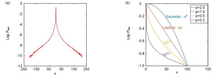
Blind deconvolution (BD) could recover a sharp image only from several degraded images. However, BD problems have the difficulties of ill-conditioned and infinite solutions, it is necessary to add prior knowledge to avoid undesired solutions. Traditional Wiener filtering based iterative blind deconvolution method assumes that the intensity of the image obeys the Gaussian distribution, while Chan et al. employ total variation prior, which assumes the gradient of the image obeys the Laplacian distribution. Given the fact that the gradient distribution of natural images is a sparse one with heavy tails, both of Gaussian and Laplacian model cannot approximate this sparse model greatly. Therefore, this paper draws on the image gradient sparse priori derived from blind motion deblurring, and applied it to the blind restoration of turbulence-degraded images.
In order to cope with the non-convex cost function caused by sparse prior, this paper uses split Bregman and look-up table method to solve effectively. Secondly, a two-step estimation strategy is adopted including kernel estimation and non-blind restoration. This paper employs the deconvolution method of Krishnan to reconstruct a sharp image with the kernel from the former step, and this strategy is essential to avoid the ringing effect reported by Fergus.
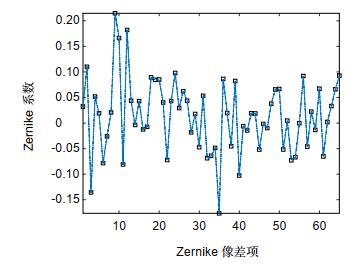
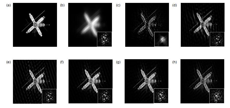
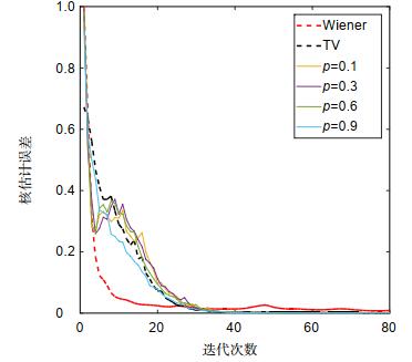
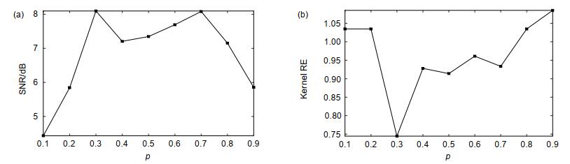
Firstly, the simulation experiment is carried out. To model the atmospheric turbulence degradation, the Zernike polynomials are used to generate the point spread function, and the OCNR5 satellite image is used as an object for observing. This paper adopts the relative error to evaluate the kernel estimation error and the signal to noise ratio (SNR) to evaluate image quality of degraded and restored ones. Both simulations and experiments on the real degraded images show that: 1) compared with the traditional Wiener filtering method and total variation prior, the sparse prior is beneficial to kernel estimation, produces sharp edges and removes ringing, thus improving the restoration quality. 2) After employing split Bregman optimization, restoration with sparse prior can converge rapidly and steadily, hence the proposed algorithm in this paper is robust and stable. 3) It is worth noting that the value of p should not be too large or too small, smaller p will amplify the noise.
-
Access History


Export File
Citation
Format
Content
 DownLoad:

-
Figure 1.
Natural images statistical model. (a) Real natural image gradient distribution; (b) Parametric model
-
Figure 2.
Simulated Zernike coefficient distribution of point spread function
-
Figure 3.
Blind deconvolution of simulated turbulence-degrade image.
-
Figure 4.
Convergence performance of algorithms
-
Figure 5.
Restored image SNRs and kernel error RE under different p values
-
Figure 6.
Real ISS restoration. (a) Degraded image; (b) Total variation restoration; (c) Sparse prior restoration with p=0.5; (d) Sparse prior restoration with p=0.1; (e) Local details of (a), (b), (c) and (d)


