
 E-mail Alert
 RSS
RSS
| Citation: |
Ma HG, Ren SL, Wei X et al. Enhanced photoacoustic microscopy with physics-embedded degeneration learning. Opto-Electron Adv 8, 240189 (2025). doi: 10.29026/oea.2025.240189

|
Enhanced photoacoustic microscopy with physics-embedded degeneration learning
-
Abstract
Deep learning (DL) is making significant inroads into biomedical imaging as it provides novel and powerful ways of accurately and efficiently improving the image quality of photoacoustic microscopy (PAM). Off-the-shelf DL models, however, do not necessarily obey the fundamental governing laws of PAM physical systems, nor do they generalize well to scenarios on which they have not been trained. In this work, a physics-embedded degeneration learning (PEDL) approach is proposed to enhance the image quality of PAM with a self-attention enhanced U-Net network, which obtains greater physical consistency, improves data efficiency, and higher adaptability. The proposed method is demonstrated on both synthetic and real datasets, including animal experiments in vivo (blood vessels of mouse's ear and brain). And the results show that compared with previous DL methods, the PEDL algorithm exhibits good performance in recovering PAM images qualitatively and quantitatively. It overcomes the challenges related to training data, accuracy, and robustness which a typical data-driven approach encounters, whose exemplary application envisions to provide a new perspective for existing DL tools of enhanced PAM.-
Keywords:
- photoacoustic microscopy /
- deep learning /
- high quality imaging /
- physical model
-

-
References
[1] Wang LV. Multiscale photoacoustic microscopy and computed tomography. Nat Photonics 3, 503–509 (2009). doi: 10.1038/nphoton.2009.157 [2] Yao JJ, Wang LV. Photoacoustic tomography: fundamentals, advances and prospects. Contrast Media Mol. Imaging 6, 332–345 (2011). doi: 10.1002/cmmi.443 [3] Yu YS, Feng T, Qiu HX et al. Simultaneous photoacoustic and ultrasound imaging: a review. Ultrasonics 139, 107277 (2024). doi: 10.1016/j.ultras.2024.107277 [4] Abdullah A, Shahini M, Pak A. An approach to design a high power piezoelectric ultrasonic transducer. J Electroceram 22, 369–382 (2009). doi: 10.1007/s10832-007-9408-8 [5] Zeng YG, Da X, Wang Y et al. Photoacoustic and ultrasonic coimage with a linear transducer array. Opt Lett 29, 1760–1762 (2004). doi: 10.1364/OL.29.001760 [6] Xu MH, Wang LV. Universal back-projection algorithm for photoacoustic computed tomography. Phys Rev E 71, 016706 (2005). doi: 10.1103/PhysRevE.71.016706 [7] Beard P. Biomedical photoacoustic imaging. Interface Focus 1, 602–631 (2011). doi: 10.1098/rsfs.2011.0028 [8] Wang LV, Gao L. Photoacoustic microscopy and computed tomography: from bench to bedside. Annu Rev Biomed Eng 16, 155–185 (2014). doi: 10.1146/annurev-bioeng-071813-104553 [9] Yao JJ, Wang LV. Photoacoustic microscopy. Laser Photonics Rev 7, 758–778 (2013). doi: 10.1002/lpor.201200060 [10] Cao R, Li J, Ning B et al. Functional and oxygen-metabolic photoacoustic microscopy of the awake mouse brain. Neuroimage 150, 77–87 (2017). doi: 10.1016/j.neuroimage.2017.01.049 [11] Wong TTW, Zhang RY, Hai PF et al. Fast label-free multilayered histology-like imaging of human breast cancer by photoacoustic microscopy. Sci Adv 3, e1602168 (2017). doi: 10.1126/sciadv.1602168 [12] Lin L, Wang LV. The emerging role of photoacoustic imaging in clinical oncology. Nat Rev Clin Oncol 19, 365–384 (2022). doi: 10.1038/s41571-022-00615-3 [13] Favazza CP, Wang LV, Jassim OW et al. In vivo photoacoustic microscopy of human cutaneous microvasculature and a nevus. J Biomed Opt 16, 016015 (2011). [14] Zhu XY, Huang Q, DiSpirito A et al. Real-time whole-brain imaging of hemodynamics and oxygenation at micro-vessel resolution with ultrafast wide-field photoacoustic microscopy. Light Sci Appl 11, 138 (2022). doi: 10.1038/s41377-022-00836-2 [15] Jeon S, Kim J, Lee D et al. Review on practical photoacoustic microscopy. Photoacoustics 15, 100141 (2019). doi: 10.1016/j.pacs.2019.100141 [16] Wu JH, Feng T, Chen Q et al. Photoacoustic guided wavefront shaping using digital micromirror devices. Opt Laser Technol 174, 110570 (2024). doi: 10.1016/j.optlastec.2024.110570 [17] Chen JB, Zhang YC, He LY et al. Wide-field polygon-scanning photoacoustic microscopy of oxygen saturation at 1-MHz A-line rate. Photoacoustics 20, 100195 (2020). doi: 10.1016/j.pacs.2020.100195 [18] Jeon S, Park J, Managuli R et al. A novel 2-D synthetic aperture focusing technique for acoustic-resolution photoacoustic microscopy. IEEE Trans Med Imaging 38, 250–260 (2019). doi: 10.1109/TMI.2018.2861400 [19] Kim C, Favazza C, Wang LV. In vivo photoacoustic tomography of chemicals: high-resolution functional and molecular optical imaging at new depths. Chem Rev 110, 2756–2782 (2010). doi: 10.1021/cr900266s [20] Telenkov SA, Alwi R, Mandelis A. Photoacoustic correlation signal-to-noise ratio enhancement by coherent averaging and optical waveform optimization. Rev Sci Instrum 84, 104907 (2013). doi: 10.1063/1.4825034 [21] Sun MJ, Feng NZ, Shen Y et al. Photoacoustic signals denoising based on empirical mode decomposition and energy-window method. Adv Adapt Data Anal 4, 1250004 (2012). doi: 10.1142/S1793536912500045 [22] Haq IU, Nagoaka R, Makino T et al. 3D Gabor wavelet based vessel filtering of photoacoustic images. In Proceedings of 2016 38th Annual International Conference of the IEEE Engineering in Medicine and Biology Society 3883–3886 (IEEE, 2016); http://doi.org/10.1109/EMBC.2016.7591576. [23] Shang RB, Archibald R, Gelb A et al. Sparsity-based photoacoustic image reconstruction with a linear array transducer and direct measurement of the forward model. J Biomed Opt 24, 031015 (2018). [24] Deng ZL, Yang XQ, Gong H et al. Two-dimensional synthetic-aperture focusing technique in photoacoustic microscopy. J Appl Phys 109, 104701 (2011). doi: 10.1063/1.3585828 [25] Chen JH, Lin RQ, Wang HN et al. Blind-deconvolution optical-resolution photoacoustic microscopy. in vivo. Opt Express 21, 7316–7327 (2013). [26] Hill ER, Xia WF, Clarkson MJ et al. Identification and removal of laser-induced noise in photoacoustic imaging using singular value decomposition. Biomed Opt Express 8, 68–77 (2016). [27] Yang CC, Lan HR, Gao F et al. Review of deep learning for photoacoustic imaging. Photoacoustics 21, 100215 (2021). doi: 10.1016/j.pacs.2020.100215 [28] Li ZS, Sun JS, Fan Y et al. Deep learning assisted variational Hilbert quantitative phase imaging. Opto-Electron Sci 2, 220023 (2023). doi: 10.29026/oes.2023.220023 [29] Saba A, Gigli C, Ayoub AB et al. Physics-informed neural networks for diffraction tomography. Adv Photonics 4, 066001 (2022). [30] Wu ZL, Kang I, Yao YD et al. Three-dimensional nanoscale reduced-angle ptycho-tomographic imaging with deep learning (RAPID). eLight 3, 7 (2023). doi: 10.1186/s43593-022-00037-9 [31] Wei X, Feng T, Huang QH et al. Deep learning-powered biomedical photoacoustic imaging. Neurocomputing 573, 127207 (2024). doi: 10.1016/j.neucom.2023.127207 [32] Gröhl J, Schellenberg M, Dreher K et al. Deep learning for biomedical photoacoustic imaging: a review. Photoacoustics 22, 100241 (2021). [33] Allman D, Reiter A, Bell MAL. Photoacoustic source detection and reflection artifact removal enabled by deep learning. IEEE Trans Med Imaging 37, 1464–1477 (2018). [34] Wang R, Zhang ZP, Chen RY et al. Noise‐insensitive defocused signal and resolution enhancement for optical‐resolution photoacoustic microscopy via deep learning. J Biophotonics 16, e202300149 (2023). doi: 10.1002/jbio.202300149 [35] Zhao HX, Ke ZW, Yang F et al. Deep learning enables superior photoacoustic imaging at ultralow laser dosages. Adv Sci 8, 2003097 (2021). doi: 10.1002/advs.202003097 [36] Vu T, DiSpirito III A, Li DW et al. Deep image prior for undersampling high-speed photoacoustic microscopy. Photoacoustics 22, 100266 (2021). doi: 10.1016/j.pacs.2021.100266 [37] He D, Zhou JS, Shang XY et al. De-noising of photoacoustic microscopy images by deep learning. arXiv: 2201.04302 (2022). https://doi.org/10.48550/arXiv.2201.04302 [38] Cheng SF, Zhou YY, Chen JB et al. High-resolution photoacoustic microscopy with deep penetration through learning. Photoacoustics 25, 100314 (2022). doi: 10.1016/j.pacs.2021.100314 [39] Zhang ZY, Jin HR, Zhang WW et al. Adaptive enhancement of acoustic resolution photoacoustic microscopy imaging via deep CNN prior. Photoacoustics 30, 100484 (2023). doi: 10.1016/j.pacs.2023.100484 [40] Gao Y, Feng T, Qiu HX et al. 4D spectral-spatial computational photoacoustic dermoscopy. Photoacoustics 34, 100572 (2023). doi: 10.1016/j.pacs.2023.100572 [41] DiSpirito A, Li DW, Vu T et al. Reconstructing undersampled photoacoustic microscopy images using deep learning. IEEE Trans Med Imaging 40, 562–570 (2021). doi: 10.1109/TMI.2020.3031541 [42] Lu JY, Zou HH, Greenleaf JF. Biomedical ultrasound beam forming. Ultrasound Med Biol 20, 403–428 (1994). doi: 10.1016/0301-5629(94)90097-3 [43] Lin HN, Cheng JX. Computational coherent Raman scattering imaging: breaking physical barriers by fusion of advanced instrumentation and data science. eLight 3, 6 (2023). doi: 10.1186/s43593-022-00038-8 [44] Zhang ZY, Jin HR, Zheng ZS et al. Deep and domain transfer learning aided photoacoustic microscopy: acoustic resolution to optical resolution. IEEE Trans Med Imaging 41, 3636–3648 (2022). doi: 10.1109/TMI.2022.3192072 [45] Dumoulin V, Visin F. A guide to convolution arithmetic for deep learning. arXiv preprint arXiv:1603.07285, 2016 [46] Krizhevsky A, Sutskever I, Hinton GE. ImageNet classification with deep convolutional neural networks. In Proceedings of the 26th International Conference on Neural Information Processing Systems 1097–1105 (Curran Associates Inc. , 2012). [47] He KM, Zhang XY, Ren SQ et al. Deep residual learning for image recognition. In Proceedings of 2016 IEEE Conference on Computer Vision and Pattern Recognition 770–778 (IEEE, 2016); http://doi.org/10.1109/CVPR.2016.90. [48] Cao Y, Xu JR, Lin S et al. GCNet: non-local networks meet squeeze-excitation networks and beyond. In Proceedings of 2019 IEEE/CVF International Conference on Computer Vision Workshops 1971–1980 (IEEE, 2019); http://doi.org/10.1109/ICCVW.2019.00246. [49] Kim T, Oh J, Kim N et al. Comparing Kullback-Leibler divergence and mean squared error loss in knowledge distillation. In Proceedings of the Thirtieth International Joint Conference on Artificial Intelligence 2628–2635 (ijcai. org, 2021). [50] Yang QS, Yan PK, Zhang YB et al. Low-dose CT image denoising using a generative adversarial network with Wasserstein distance and perceptual loss. IEEE Trans Med Imaging 37, 1348–1357 (2018). doi: 10.1109/TMI.2018.2827462 [51] Wang ZY, Zhou YF, Hu S. Sparse coding-enabled low-fluence multi-parametric photoacoustic microscopy. IEEE Trans Med Imaging 41, 805–814 (2022). doi: 10.1109/TMI.2021.3124124 [52] Zhang YC, Chen JB, Zhang J et al. Super‐low‐dose functional and molecular photoacoustic microscopy. Adv Sci 10, 2302486 (2023). doi: 10.1002/advs.202302486 [53] Siregar S, Nagaoka R, Haq IU et al. Non local means denoising in photoacoustic imaging. Jpn J Appl Phys 57, 07LB06 (2018). doi: 10.7567/JJAP.57.07LB06 [54] Frangakis AS, Hegerl R. Noise reduction in electron tomographic reconstructions using nonlinear anisotropic diffusion. J Struct Biol 135, 239–250 (2001). doi: 10.1006/jsbi.2001.4406 [55] Gauthier J. Conditional generative adversarial nets forconvolu-tional face generation. Class project for Stanford CS231N: con-volutional neural networks for visual recognition. WinterSemester 2014, 2 (2014). [56] Ronneberger O, Fischer P, Brox T. U-Net: convolutional networks for biomedical image segmentation. In Proceedings of the 18th International Conference on Medical Image Computing and Computer-Assisted Intervention 234–241 (Springer, 2015); http://doi.org/10.1007/978-3-319-24574-4_28. [57] Ma HG, Yu YS, Zhu YH et al. Monitoring of microvascular calcification by time-resolved photoacoustic microscopy. Photoacoustics 41, 100664 (2025). doi: 10.1016/j.pacs.2024.100664 -
Supplementary Information
Supplementary information for Enhanced photoacoustic microscopy with physics-embedded degeneration learning 
-
Access History
Figures(10)
Tables(2)
Article Metrics

Export File
Citation
Ma HG, Ren SL, Wei X et al. Enhanced photoacoustic microscopy with physics-embedded degeneration learning. Opto-Electron Adv 8, 240189 (2025). doi: 10.29026/oea.2025.240189
Format
Content
 DownLoad:
-
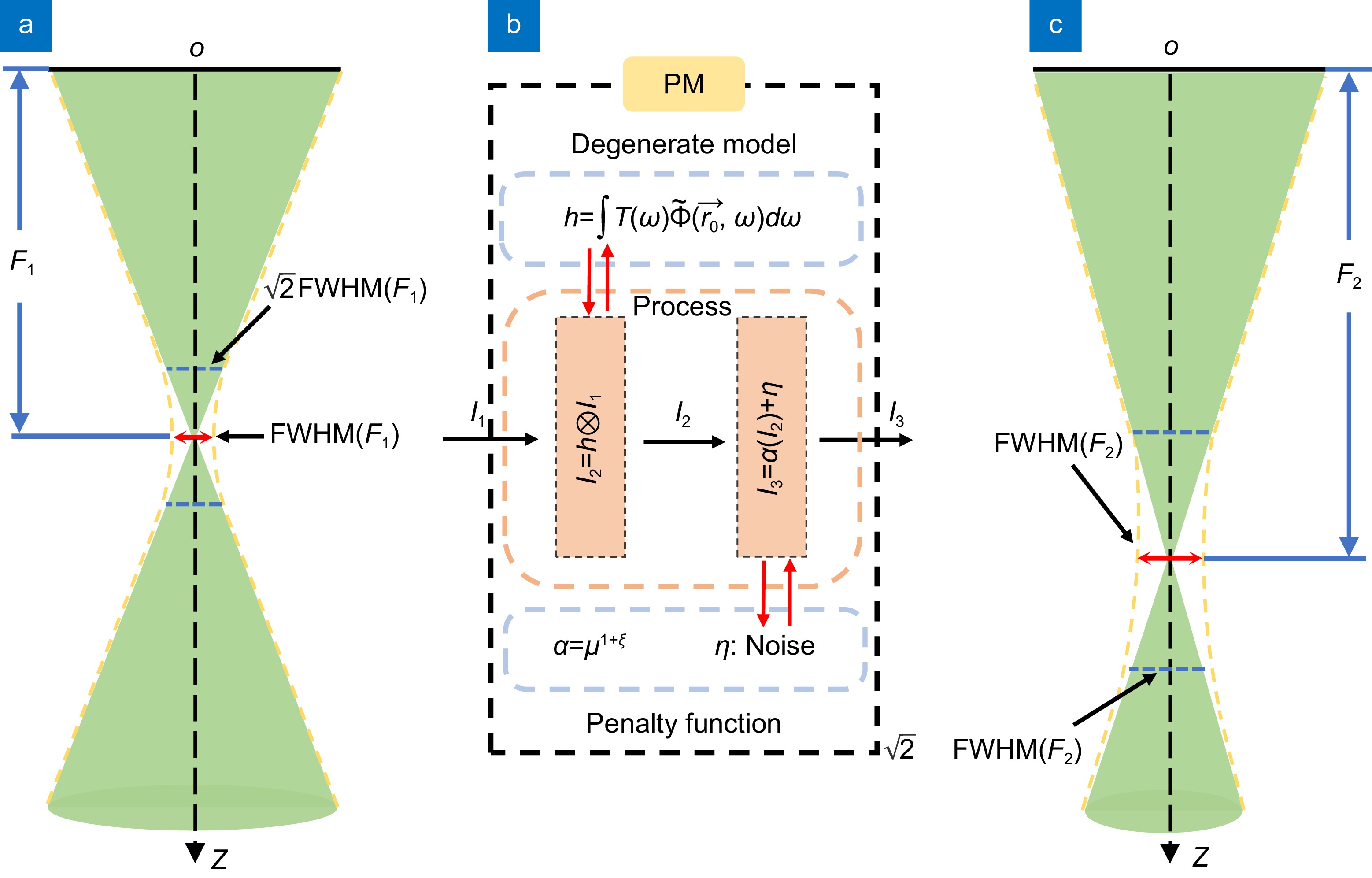
Figure 1.
Schematic diagram of physical mechanism. (a) Field pattern of the transducer at a shallower focal plane. (b) A simple schematic of the physical model. (c) Field pattern of the transducer at a deeper focal plane.
-
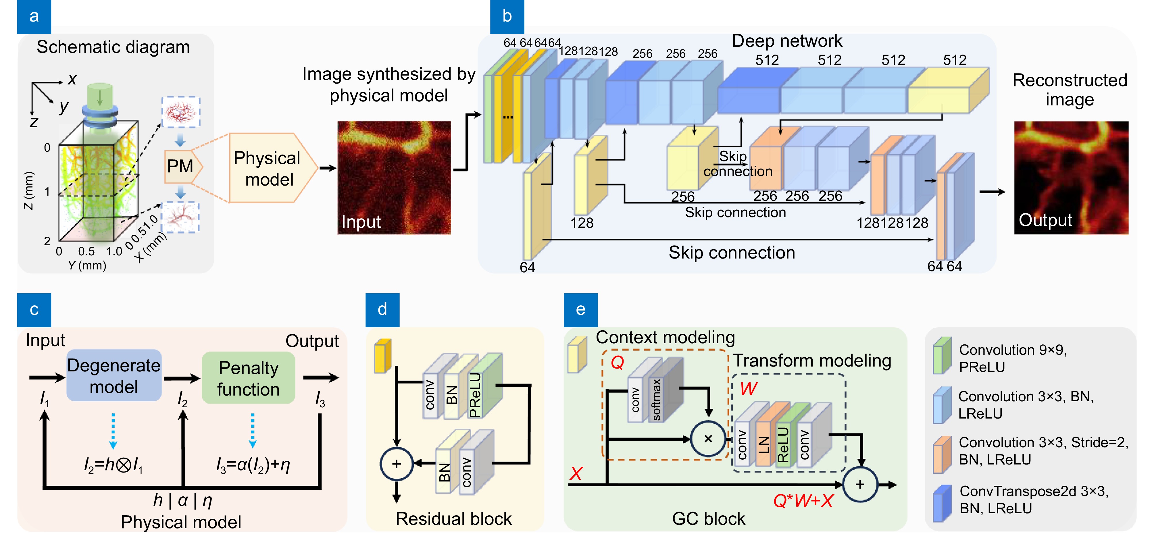
Figure 2.
Network structure and flow chart. (a) Schematic diagram of the physical model. (b) Basic structure diagram of the proposed network. (c) Image generation process of the physical model. (d) Residual module. (e) GC attention module.
-
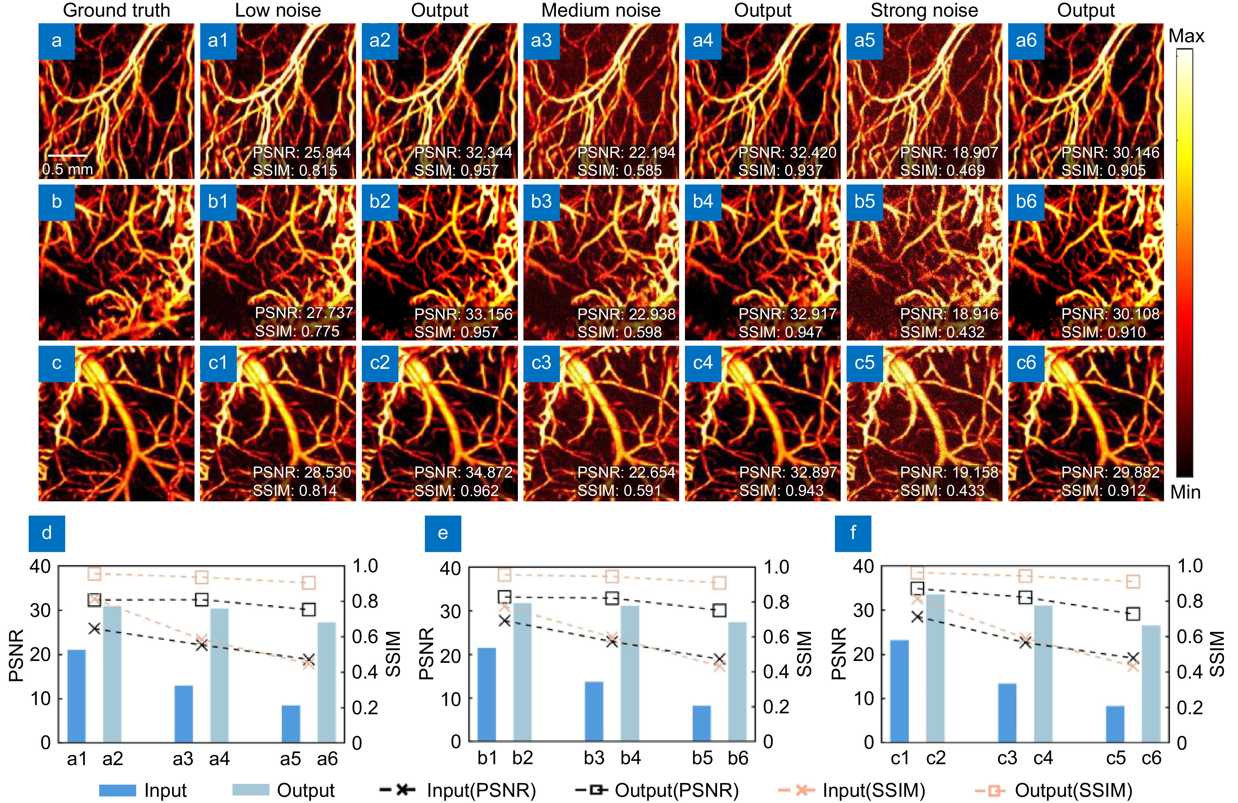
Figure 3.
Processing effect diagram of different noises. (a−c) are the ground truth images of three different tests. (a1−c1, a3−c3, a5−a5) are the low noise, medium noise, and high noise images of the three different tests, respectively. (a2–c2, a4–c4, a6–c6) are the images output by the network for the three different test images. (d−f) are the data analyses of the three test images, with PSNR on the left and SSIM on the right, and the bar chart showing the product of PSNR and SSIM weights.
-
Figure 4.
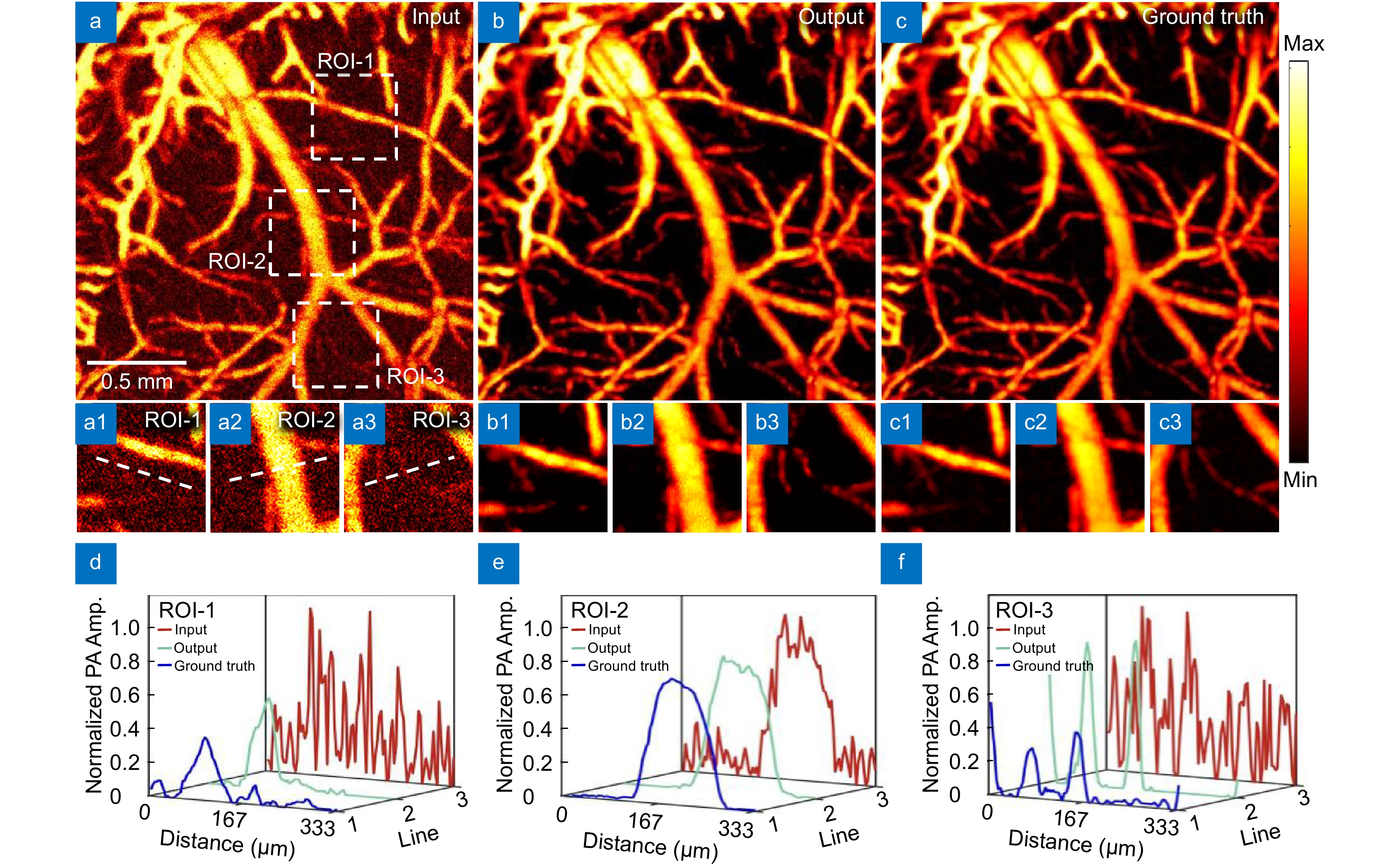
Effect diagram under strong noise. (a) Image input with strong noise. (b) Network reconstruction result. (c) Ground truth image; (a1−a3, b1−b3, c1−c3) are the magnified images of the corresponding ROI regions. (d) Maximum intensity projection analysis along the line in ROI-1. (e) Maximum intensity projection analysis along the line in ROI-2. (f) Maximum intensity projection analysis along the line in ROI-3.
-
Figure 5.
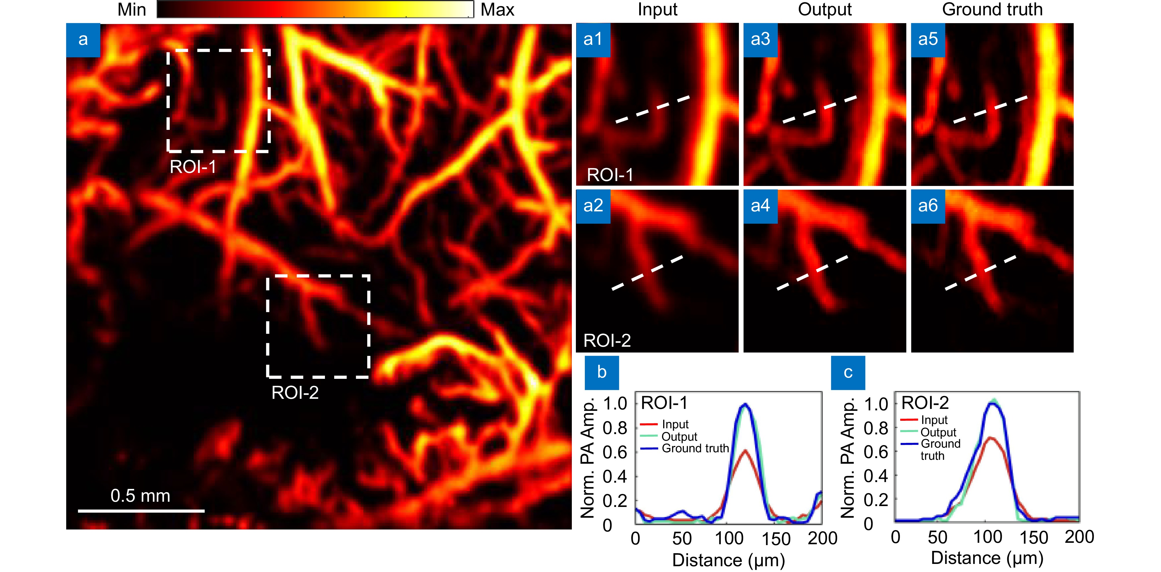
Resolution enhancement effect diagram. (a) Severely degraded, noise-free image input. (a1–a2) are magnified images of the ROI regions of the input images. (a3–a4) are magnified images of the ROI regions of the output images. (a5–a6) are magnified images of the ground truth ROI regions. (b) Maximum intensity projection analysis along the line in ROI-1. (c) Maximum intensity projection analysis along the line in ROI-2.
-
Figure 6.
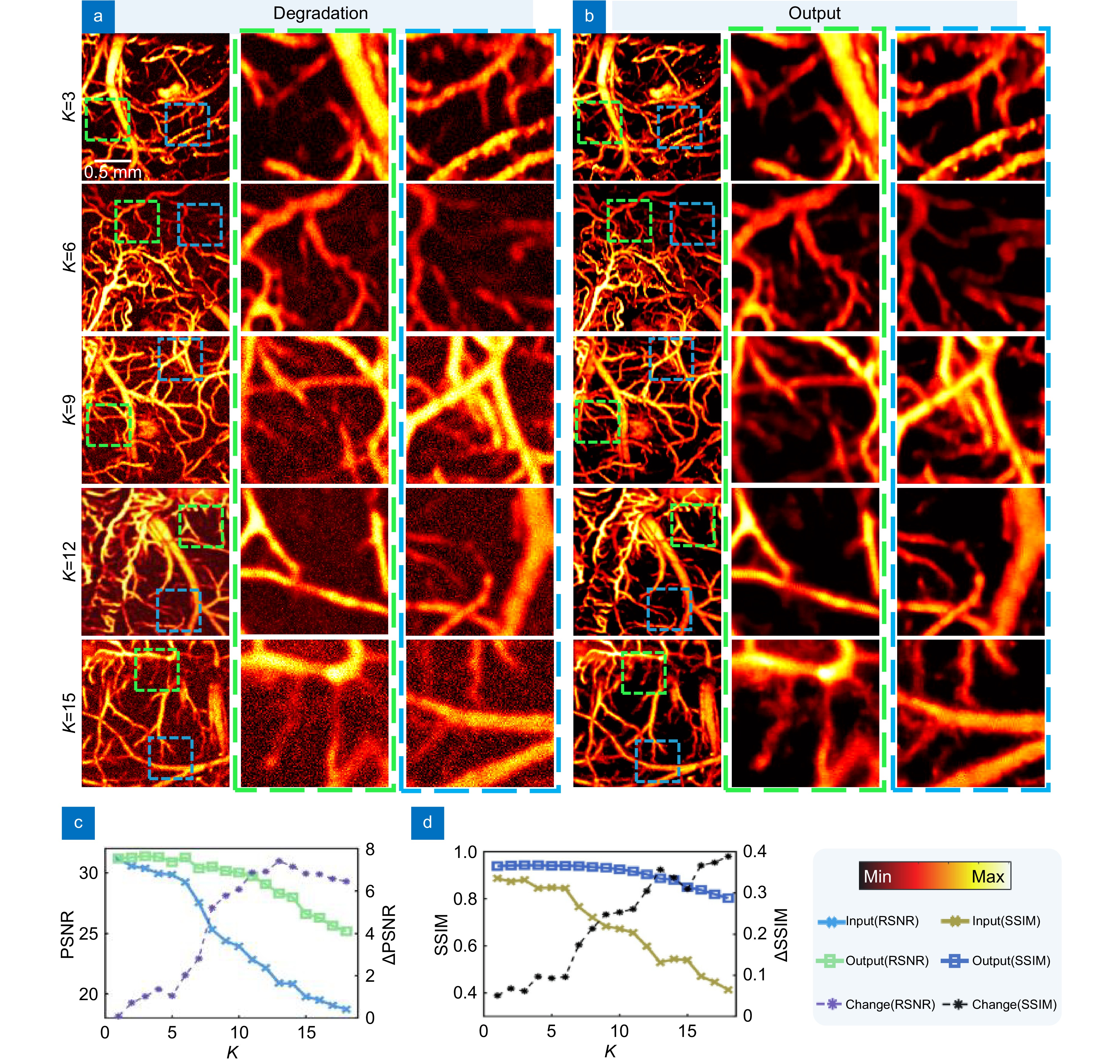
Reconstructed images with different degeneration effects. (a) Images under different degeneration models. (b) Results of different degeneration models after network output. (c) PSNR feature analysis for different degradation models, where ΔPSNR represents the difference in PSNR between the input and output. (d) SSIM feature analysis for different degradation models, where ΔSSIM represents the difference in SSIM between the input and output.
-
Figure 7.
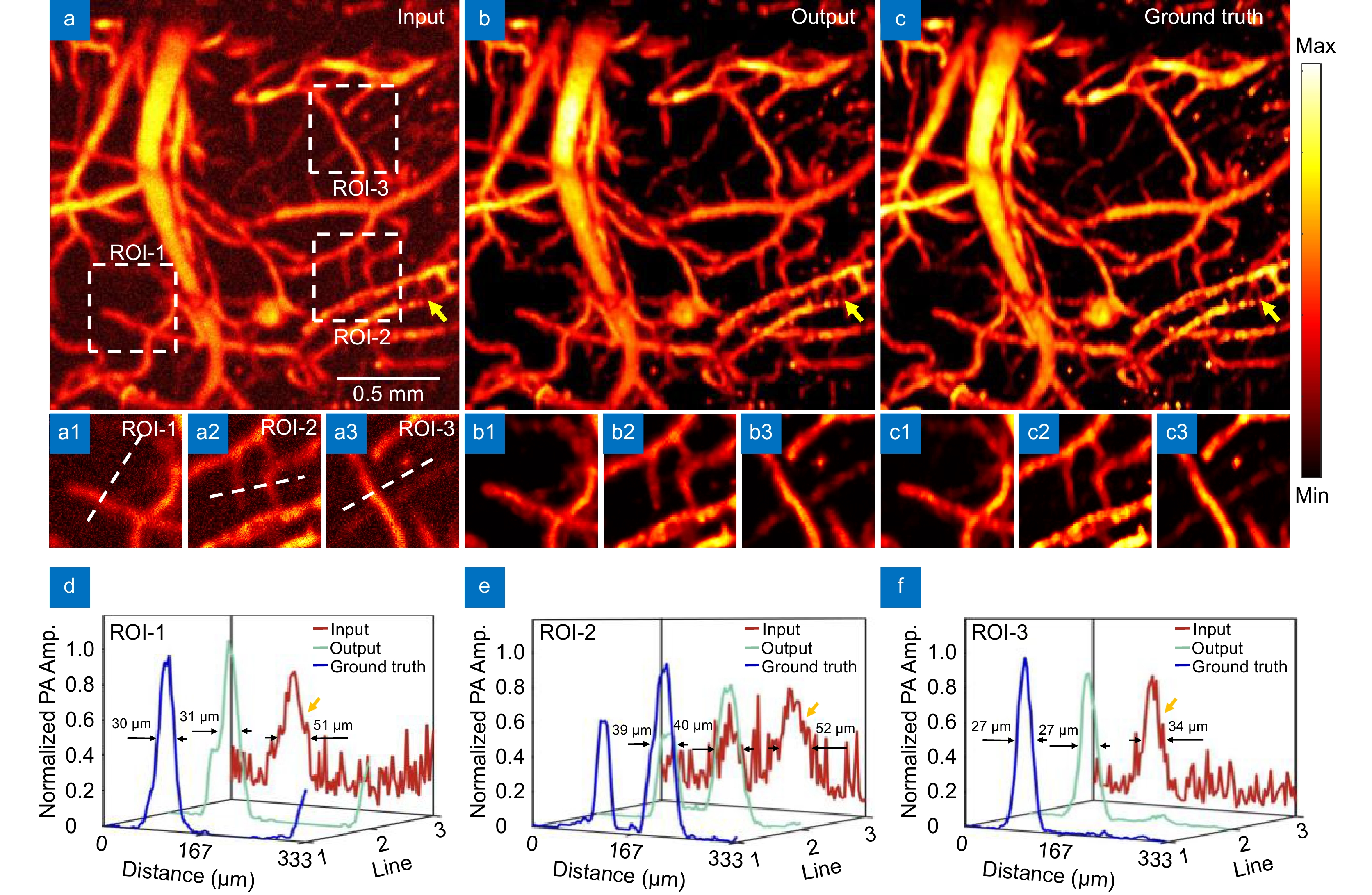
Reconstruction effect diagram under high degeneration. (a) Input images with severe degeneration. (b) Network reconstruction results. (c) Ground truth images. (a1–a3), (b1–b3), (c1–c3)(a1-a3,ba-b3,c1-c3) are the magnified images of the corresponding ROI regions. (d) Maximum intensity projection analysis along the line in ROI-1. (e) Maximum intensity projection analysis along the line in ROI-2. (f) Maximum intensity projection analysis along the line in ROI-3.
-
Figure 8.
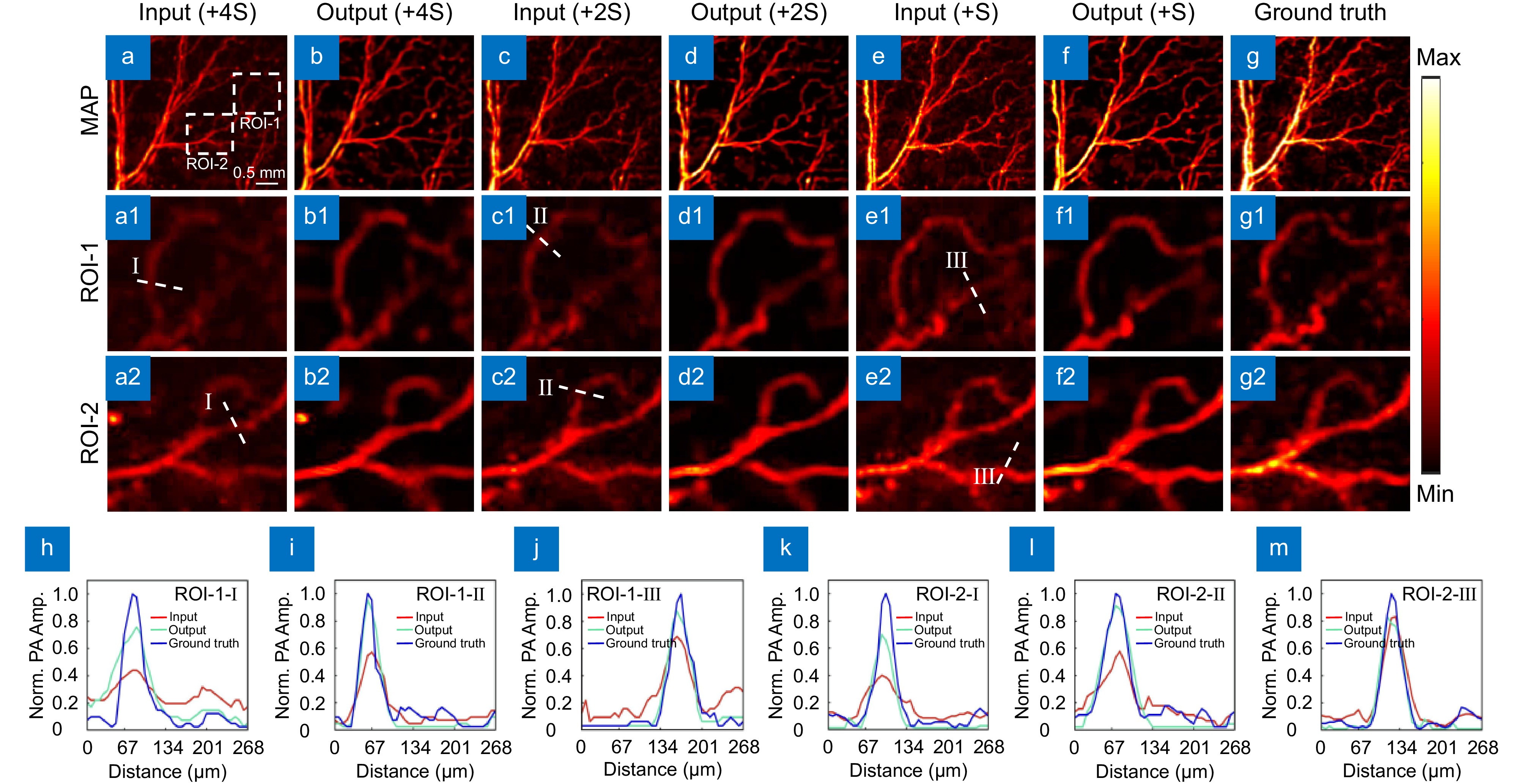
Imaging effect and reconstruction results at varying thickness levels. (a−b) Photoacoustic microscopy images and corresponding network output for four silicone layers. (c−d) Photoacoustic microscopy images and network output for two silicone layers. (e−f) Photoacoustic microscopy images and network output for one silicone layer. (g) Photoacoustic microscopy image with no silicone sheet added. (a1–g1, a2–g2) Magnified views of two ROI regions in the input images. (h−j) Maximum intensity projection analysis along the line in the magnified images of ROI-1. (k−m) Maximum intensity projection analysis along the line in the magnified images of ROI-2.
-
Figure 9.
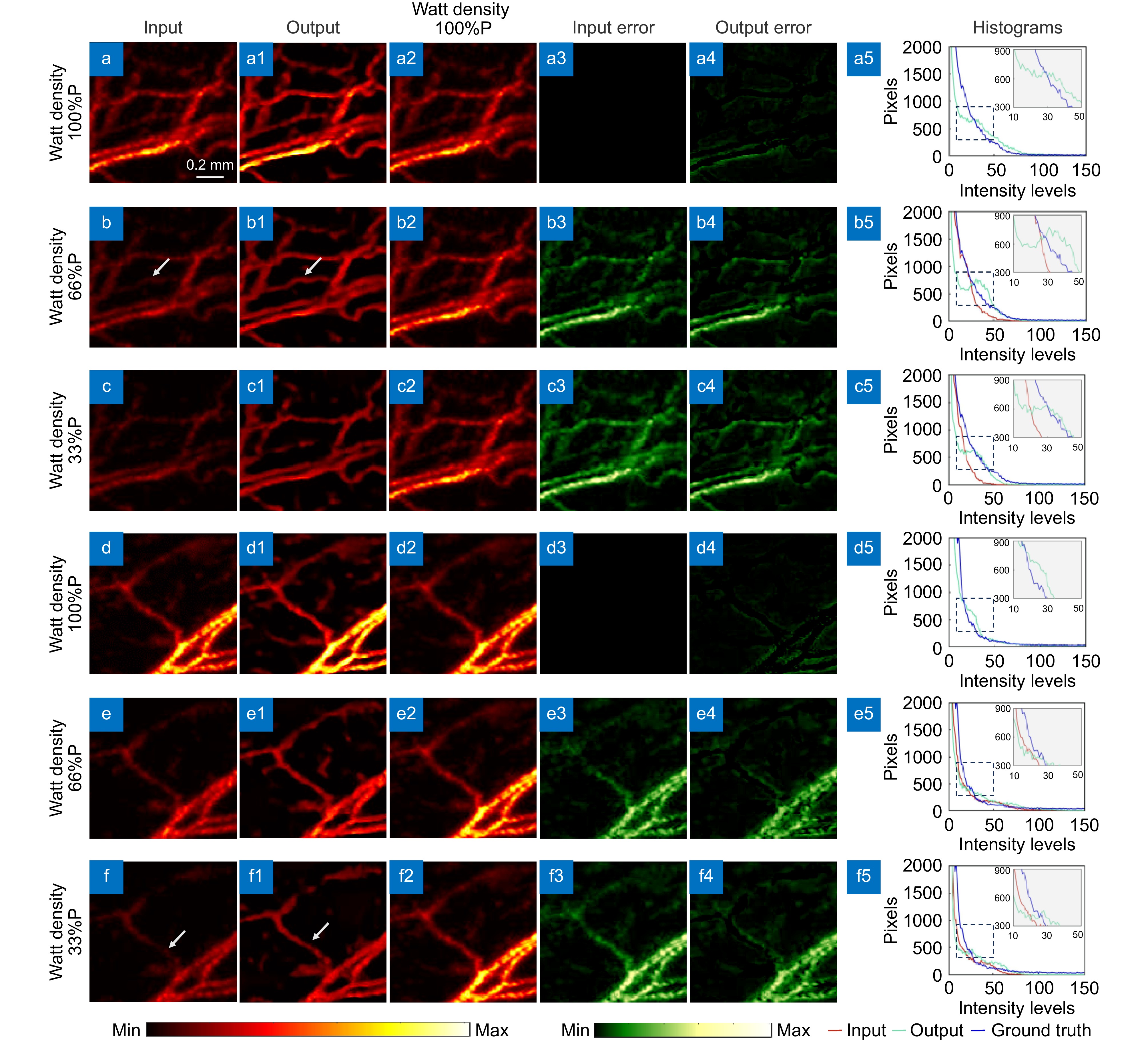
Effect diagram and reconstruction diagram under different laser energy. (a−f) Photoacoustic microscopy images at 100%, 66%, and 33% power, respectively. (a1–f1, a2–f2) Correspond to the network output images of the input images and the photoacoustic images obtained at 100% power. (a3–f3, a4–f4) Correspond to the error maps of the input and output images compared to the images obtained at 100% power. (a5–f5) Histograms of the input images, output images, and images obtained at 100% power.
-
Figure 10.
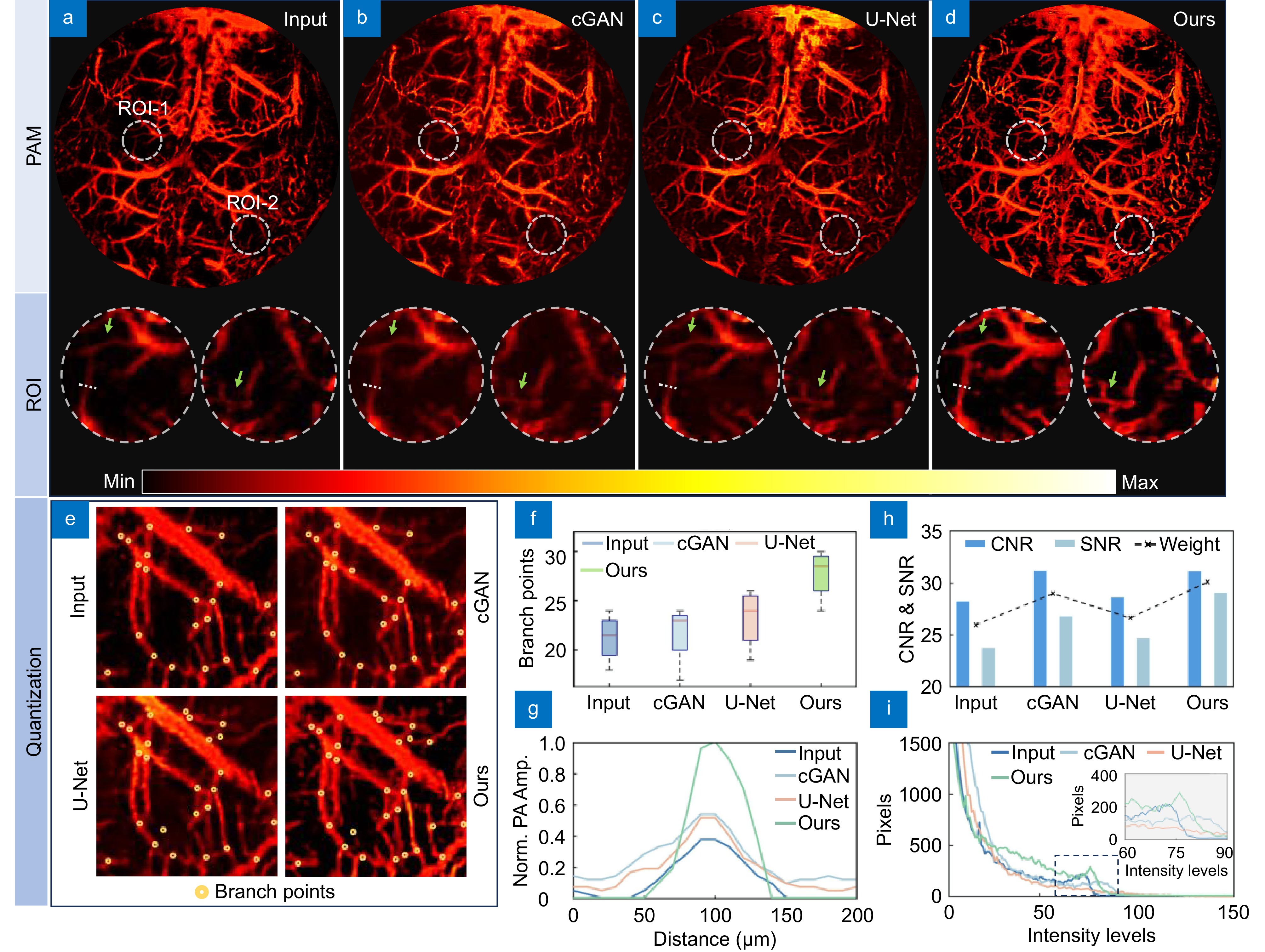
Different methods of brain reconstruction in mice. (a−d) Input images, photoacoustic microscopy images generated by cGAN, U-Net, and our network, respectively. (e) Blood vessel branch marking images of input and output images using cGAN, U-Net, and our network methods. (f) Error analysis of blood vessel branch markings. (g) Maximum intensity projection analysis of the dashed line in ROI area. (h) Comparison of Contrast-to-Noise Ratio (CNR), SNR, and their weights between input images and the three methods. (i) Histogram analysis of input images and the three methods.


